Introduction

In the last article we looked at how attention can be used with recurrent neural networks (RNNs) to generate a sequence from an input sequence. Specifically, we looked at the problem of translating an input sequence from one language into another. We saw that with RNNs without attention, the decoder in a translation model must use a single context vector to compress all the information in the source sequence; with attention, we can attend to different tokens at different decoder timesteps, which enables the model to “pay attention to” different things at different timesteps. This seems intuitively helpful, since if we’re translating a sequence, only certain parts of the sequence are relevant at certain decoding timesteps. Let’s revisit the attention weights example from part 1.

This figure shows the attention weights from each of the predicted tokens on the left to the source tokens on the right. Each generated token on the left attends to each source token on the right, and the sum of weights from each generated token add up to 1. Hover over each line to see the weights between tokens more easily. Only weights > 0.1 are being shown for ease of viewing.

At the first timestep, we pay attention to the end of sequence token </s>, which indicates that we need to start the translation, and we output <s>, the start of sequence token.

At the second timestep we pay attention to “But” and look forward 1 timestep to “why” and output the French word for “but,” “Mais.”

The transformer builds on the idea of attention and uses attention as feature extraction. It was first introduced in the paper (Vaswani et al., 2017).

In Weaknesses of RNN architecture I’ll motivate the need for the transformer architecture. In Transformer architecture I’ll go more in depth into its architecture. Finally, in Experiments and results I’ll show how the transformer performance compares to the RNN performance, and as a sub-research question, how the original encoder-decoder transformer architecture compares to GPT-style decoder-only architecture in Encoder-decoder vs decoder-only

For this post, it helps if you have read the previous post or are already familiar with this topic.

All code/trained weights, data for this post can be accessed here

Weaknesses of RNN architecture

sequential processing

Recall that in the RNN we extract features from the input sequence iteratively.

To repeate the example from the previous post:

Let’s tokenize the sentence as [“I”, “have”, “socks”, “.”]

Let the embedding vector be $x \in \mathbb{R}^2$

Let the hidden state be $h \in \mathbb{R}^3$.

The RNN works by iteratively processing each token in the input sequence. We start with an initial “hidden state” defined by h_t. When we process each token, we use the current hidden state h_t and the current token x_t as input to update the hidden state. In this way we can keep track of what we have seen so that the model can encode the meaning of the entire sequence. The hidden state can be seen as an internal representation of the sequence, including token x_t and is collected in the variable outs. outs therefore can be seen as a $\mathbb{R}^{T\times h}$ encoded representation of the sequence, and h_t as the final representation of the entire sequence.

We had to process each token iteratively in order for an arbitrary token $x_{t}$ to “know about” a previous token $x_{t'}$. Iterative processing should be avoided if possible, since we would like to make use of the parallel processing that modern GPUs provide.

The transformer does not use iterative processing to encode an input sequence but instead uses an attention mechanism so that in parallel, all tokens can “know about” all other previous tokens.

Only a single attention vector

In the RNN with attention, we are only calculating an alignment vector between $q$ and $K$ a single time, producing a single measure of similarity, or alignment, between the question $q$ and the keys $K$. What if we wanted to align the query with the keys in multiple different ways, for example, by looking for nouns, verbs, adjectives, proper nouns, etc. separately. Currently, using a single measure of similarity, these ideas of similarity are all combined into a single measure, which might make it harder for the model to learn complex patterns.

The transformer uses multiple heads of attention to achieve this.

Only a single layer of attention

In the RNN with attention we stack multiple RNNs together to achieve depth but just calculate attention between the outputs. We’d like to instead add more layers to the attention calculation. We know that in deep learning, depth can allow us to learn more complex patterns.

Transformer architecture

The paper that first introduced the transformer architecture, (Vaswani et al., 2017) is called “Attention is all you need.” From that title we might guess that the transformer makes attention a core component of the architecture. Whereas with the RNN with attention we use attention to align the decoder hidden state with the encoder outputs, but still use sequential recurrent processing using $h_t = f(h_t, x_t; W)$ to update the hidden state, with the transformer we remove the recurrent hidden state calculation and instead calculate attention as the main computational unit and feature extractor.

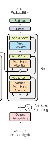
The transformer has many other components, including attention that already existed at the time, and combines them into a novel architecture. Let’s look at the diagram of the architecture from the paper that introduced the transformer:

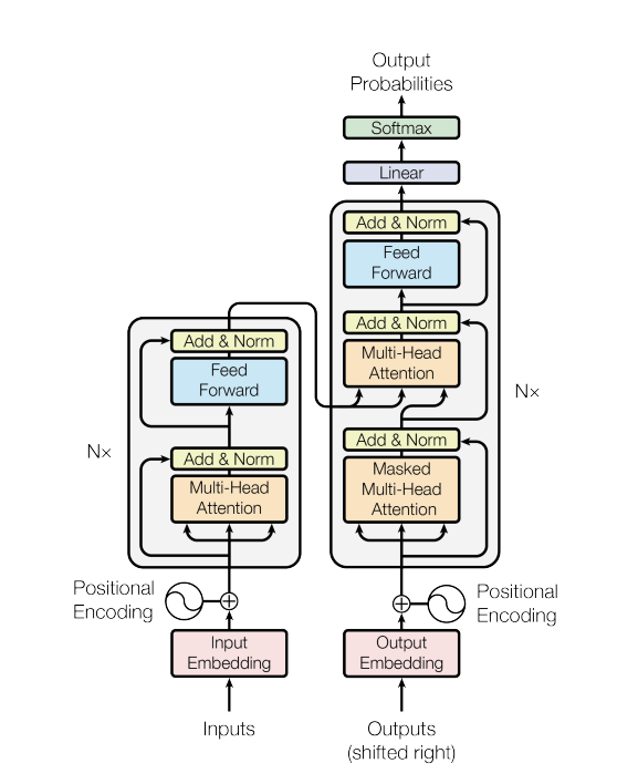
On the left of the diagram is the encoder, and on the right is the decoder. The encoder encodes the source sentence while the decoder generates the translated sentence using the encoded representation as input. The encoder and decoder are largely the same with a few differences.

We’ll look at each component in the diagram and start with the encoder.

how transformer uses attention

In the encoder, the RNN uses a recurrent hidden state that takes as input the current token $x_t$ and the previously seen tokens are encoded using the hidden state $h_t$. This is a sequential operation since we iterate through each token in the sequence. How can this be replaced with a similar operation without iterating through each token?

We’ve seen how attention can be computed between the RNN decoder hidden state vector and the encoder outputs; the decoder hidden state is treated as the query $q$, and the encoder outputs are treated as the keys $K$. The transformer adapts attention by generalizing it to an arbitrary number of queries and keys. In the transformer encoder, we calculate attention not just between a single vector and a set of keys, but between a set of query vectors and a set of keys. The set of query vectors $Q$ is the entire source sequence, and the set of keys is the entire source sequence. The queries and the keys are the same! This is known as self-attention. Let’s look at self-attention in detail.

First, though, we need to convert the tokens into numeric vectors as with the RNN, which is the which is the Input
Embedding box in the diagram, and is the same as described in the previous post.

self-attention

Step 1: Q, K, V projection

Now, we can start to compute self-attention, which is the Multi-Head
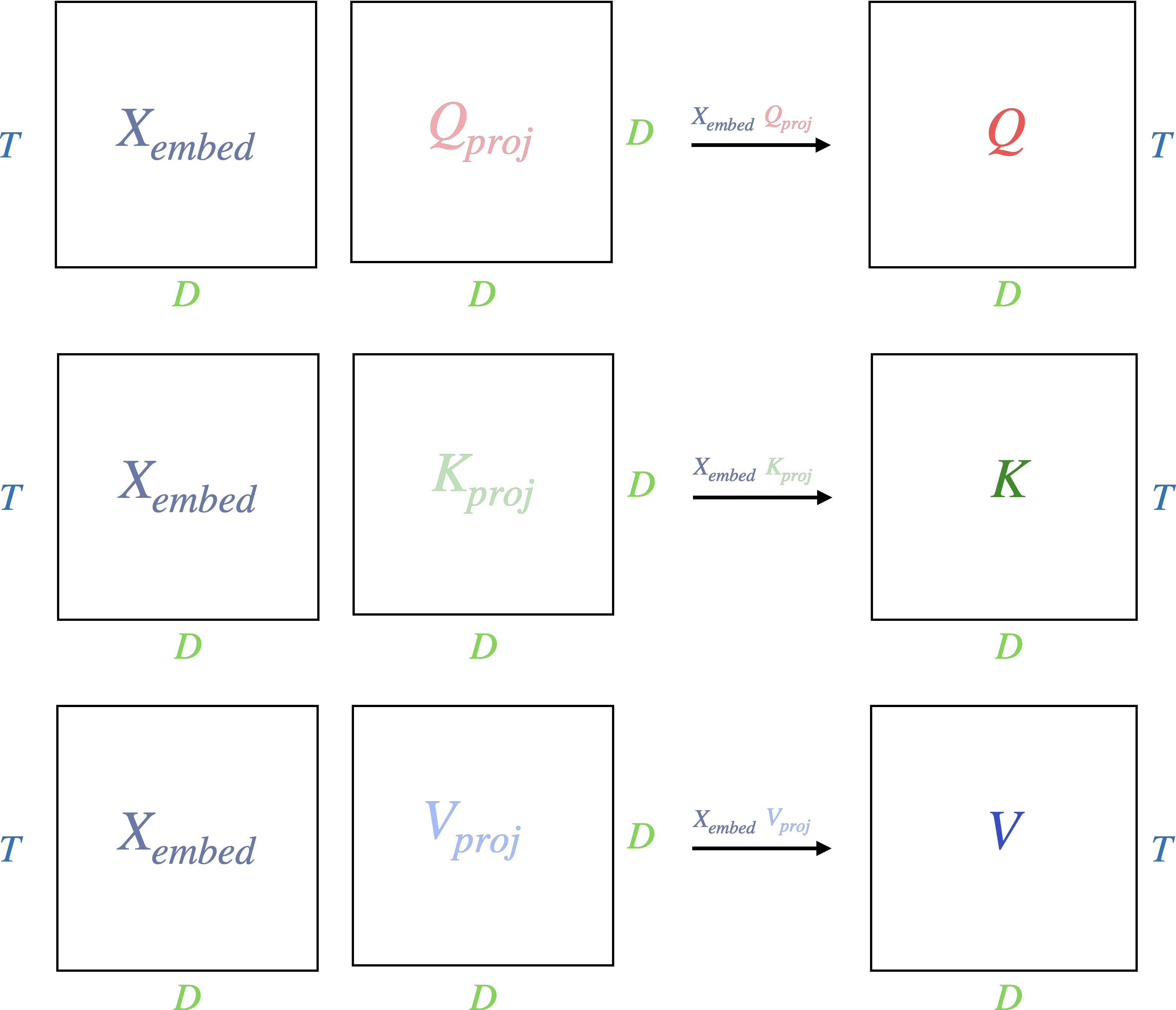
Attention box in the diagram. First, we project the sequence embedding matrix 3 times using 3 different linear maps, $Q_{proj} \in \mathbb{R}^{D \times D}$, $K_{proj} \in \mathbb{R}^{D \times D}$, and $V_{proj} \in \mathbb{R}^{D \times D}$. This results in three new tensors, $Q$, $K$, and $V$, all size $T \times D$. These are the queries, keys, and values respectively.

Importantly, notice that we reuse the same sequence to produce the queries, keys, and values. We do not use different sequences as in the RNN with attention.

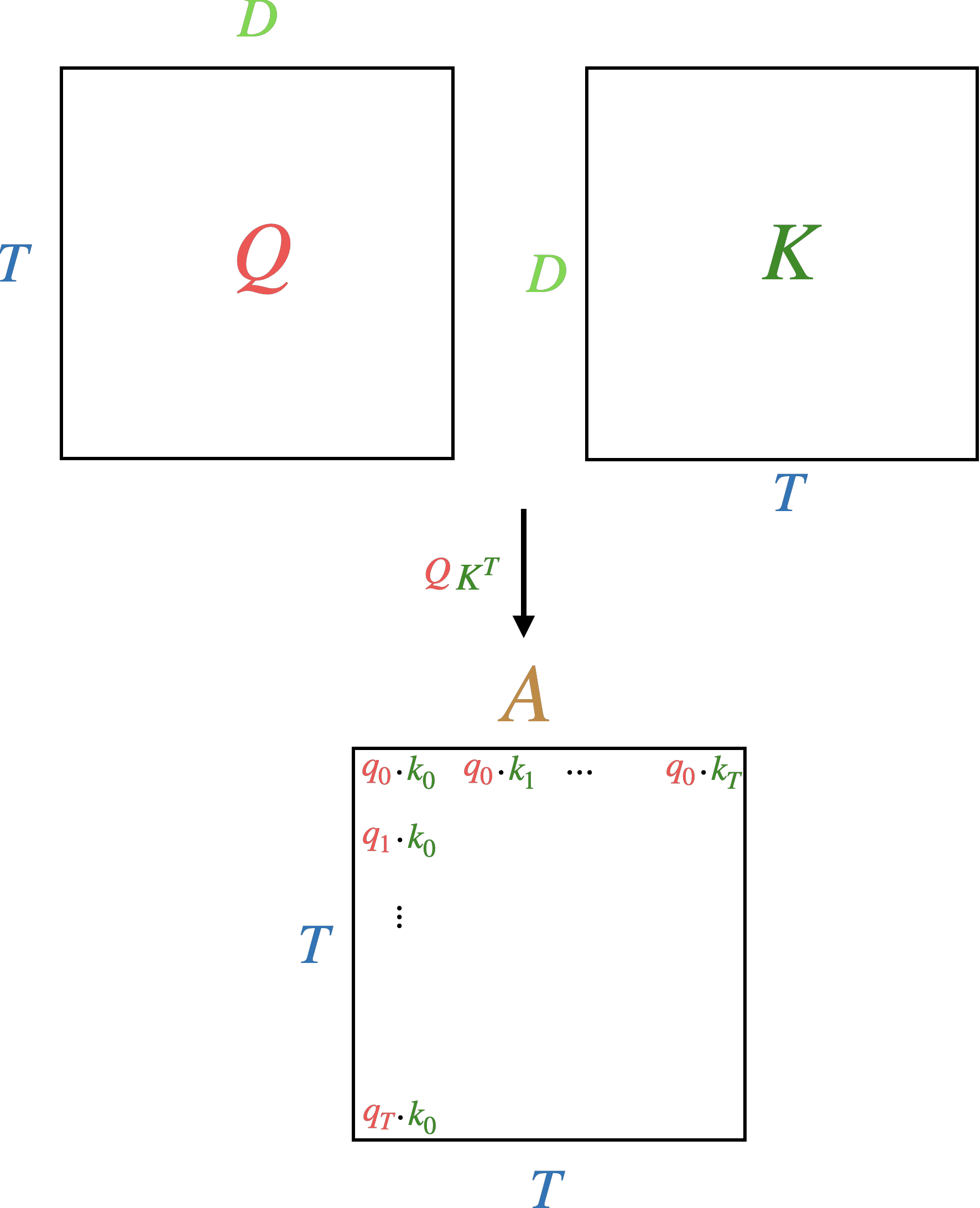
Figure 3: Query, keys, and values projections

Step 2: attention weights

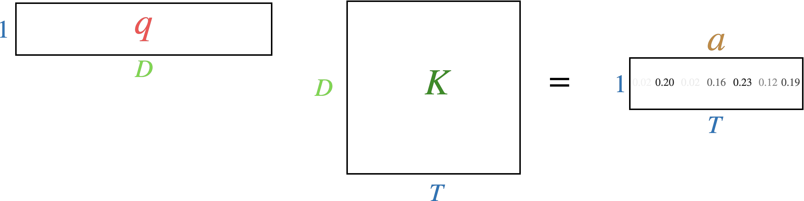
We then compute the attention weights, $A$. These are calculated the same way as in RNN with attention, using the dot product between a query $q$ and key $k$. However, in the transformer there is not just one query (as was the case with the decoder hidden state in the RNN with attention) but $T$ queries and $T$ keys. In other words, we treat each token as both a query and key, so that we have $T$ queries and $T$ keys each of dimension $D$. We then calculate similarity using dot-product (aka cosine similarity) between all queries and all keys in parallel using matrix multiplies. This results in a $T \times T$ matrix including the similarity between every query-key combination.

attention 1 — Figure 4: Query and key similarity

Note:

Note the implications of storing a $T \times T$ matrix. Here $T$ is known as the context length. It is the maximum length the model can take as input and hold in memory. The model then requires $O(T^2)$ memory to store attention weights. This can get expensive as $T$ gets larger. If the context length is $1024$ which is small for LLMs, then the $T \times T$ matrix will store over $1M$ numbers. Before with the RNN with attention, we never explicitly stored the $T \times T$ matrix because we iterated through the tokens sequentially and maintained a hidden state. But we said that this was not scalable because it requires sequential iteration. With the transformer we’ve parallelized extracting information from the sequence and so have more efficient compute but at the cost of greater memory needs.

As before, we divide each product by $\sqrt{D}$ as explained in the previous post. Finally, we use the ${softmax}$ function for each query across all keys to make positive and normalize to a probability distribution. ${softmax}(A_{ij})$ is defined as:

\[\text{softmax}(A_{ij}) = \frac{\exp(A_{ij})}{\sum_{k=1}^{T} \exp(A_{ik})}, \quad i,j = 1,\dots, T.\]

This gives us a measure of similarity between each query and key, which is in the range $[0, 1]$ and sums to 1 across keys for a given query.

Note that we use the terminology $q_i$ “attends to” $k_j$ to denote a strong similarity between $q_i$ and $k_j$.

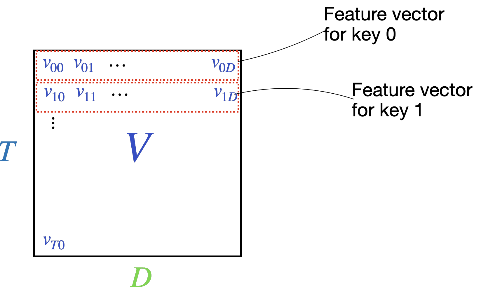
Step 3: weighting features

The matrix $V$ contains feature vectors of length $d$ for each of the $k$ keys. Row $0$ contains a $d$-dimensional vector for key $0$, row 1 a $d$-dimensional vector for key $1$, etc.

We’d like to weight each feature vector by the attention weights by multiplying the attention matrix $A$ with the feature matrix $V$.

example

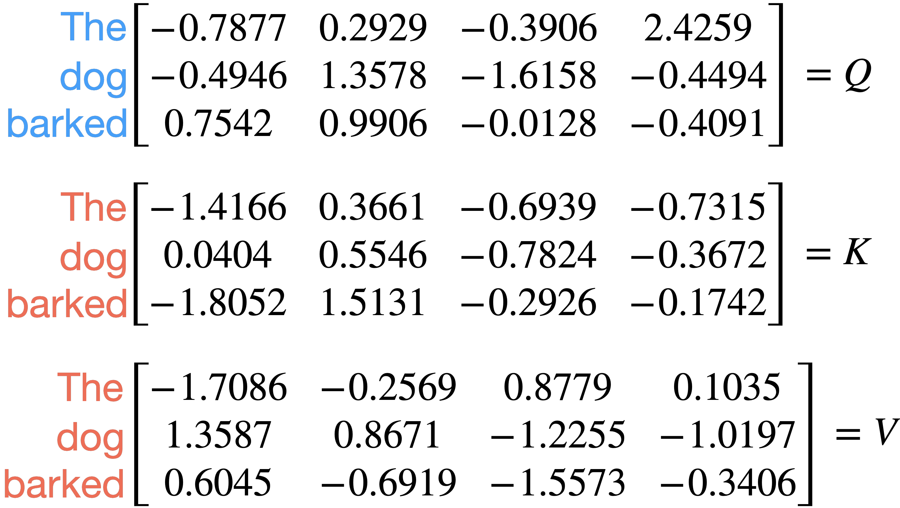
Let’s look at a concrete example using the sequence “The dog barked” and for simplicity let’s tokenize as ["The", "dog", "barked"]. Let $D$ be 4.

Let denote a value for a query and denote a value for a key and $Q$, $K$ and $V$ be:

$A$ is:

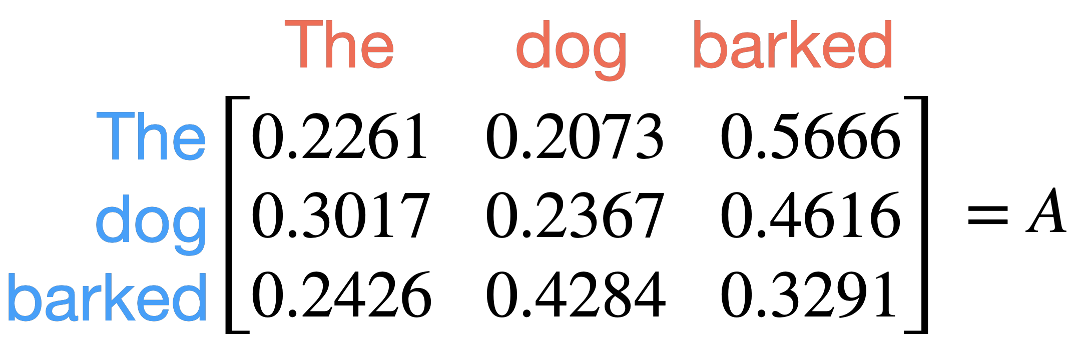
This shows that the token “The” paid attention most strongly to “barked”, “dog” to “barked” and “barked” to “dog”.

Next we compute $AV$:

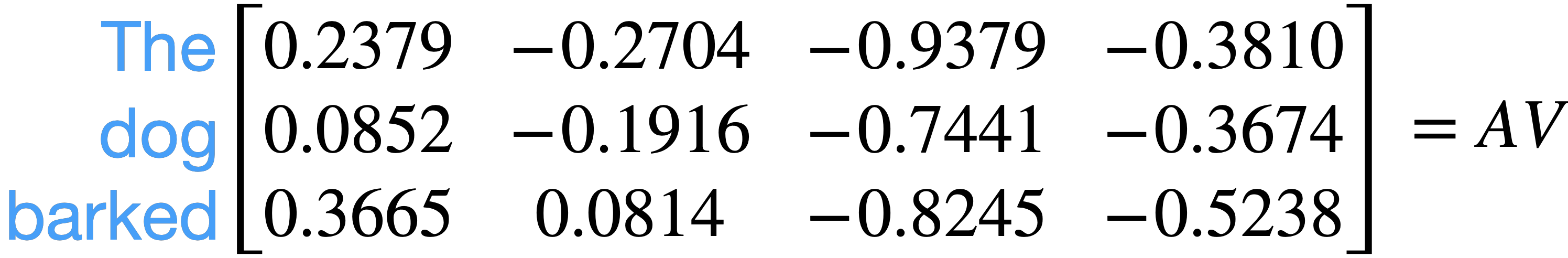
If we look at the weighted feature vector for barked:

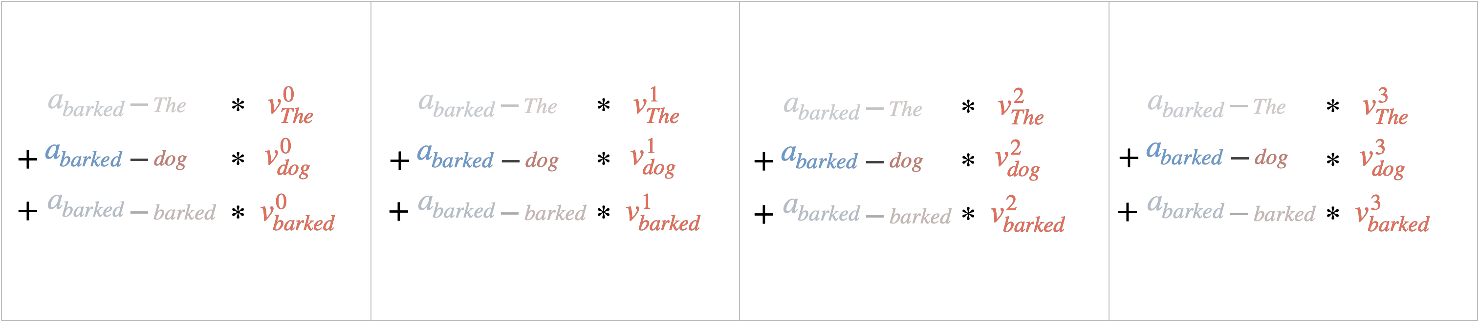
We see that because the attention $a_{barked-dog}$ is the strongest, that the feature vector $v_{dog}$ is given the most weight when calculating the weighted feature vector for barked.

Also note that the weighted feature vector for barked now includes information from all other keys in the sequence.

multi-headed attention

We said that one of the downsides to the RNN with attention was that the decoder hidden state could only ask one “question” of the encoded source sequence. This is because $qK^T$ results in a $T$-dimensional vector $a$ representing the attention weights. The hidden state only asks a single “question” which gets ranked as a probability distribution against the $T$ keys in the encoder output.

The same is true of the attention mechanism in steps 1 through 3 above. Each token or (“query”) only asks a single question of every other token (“key”). What if we want each token to be able to ask multiple questions of the other tokens and rank alignment for each question separately. These “questions” are learned by the model, but presumably different questions would be “is this an adjective?” or “is this a proper noun?” We can see examples of what kinds of different questions the model has learned to ask in attention examples.

How can we improve the attention mechanism so that each token asks multiple different questions instead of just a single question? Recall that we map each token to a $T \times D$ tensor $Q$, and separately map to a different $T \times D$ tensor $K$. To calculate attention, we take the product $QK^T$ to produce a $T \times T$ tensor of attention weights, normalized so that each query’s attention maps to a probability distribution for each key. Each query only asks a single question of each key.

To improve this so that each query can ask multiple questions of each key, we need to compute multiple $T \times T$ attention tensors for each question. The number of questions is called $H$ and is a hyperparameter. Each $h$ is called a “head” and this strategy is called “multi-head attention.”

To construct multiple heads, we split $Q$, $K$, and $V$, all of which are $\mathbb{R}^{T \times D}$ respectively into $\mathbb{R}^{T \times H \times D/H}$ tensors, which is equivalent in original size to a $\mathbb{R}^{T \times D}$ tensor.

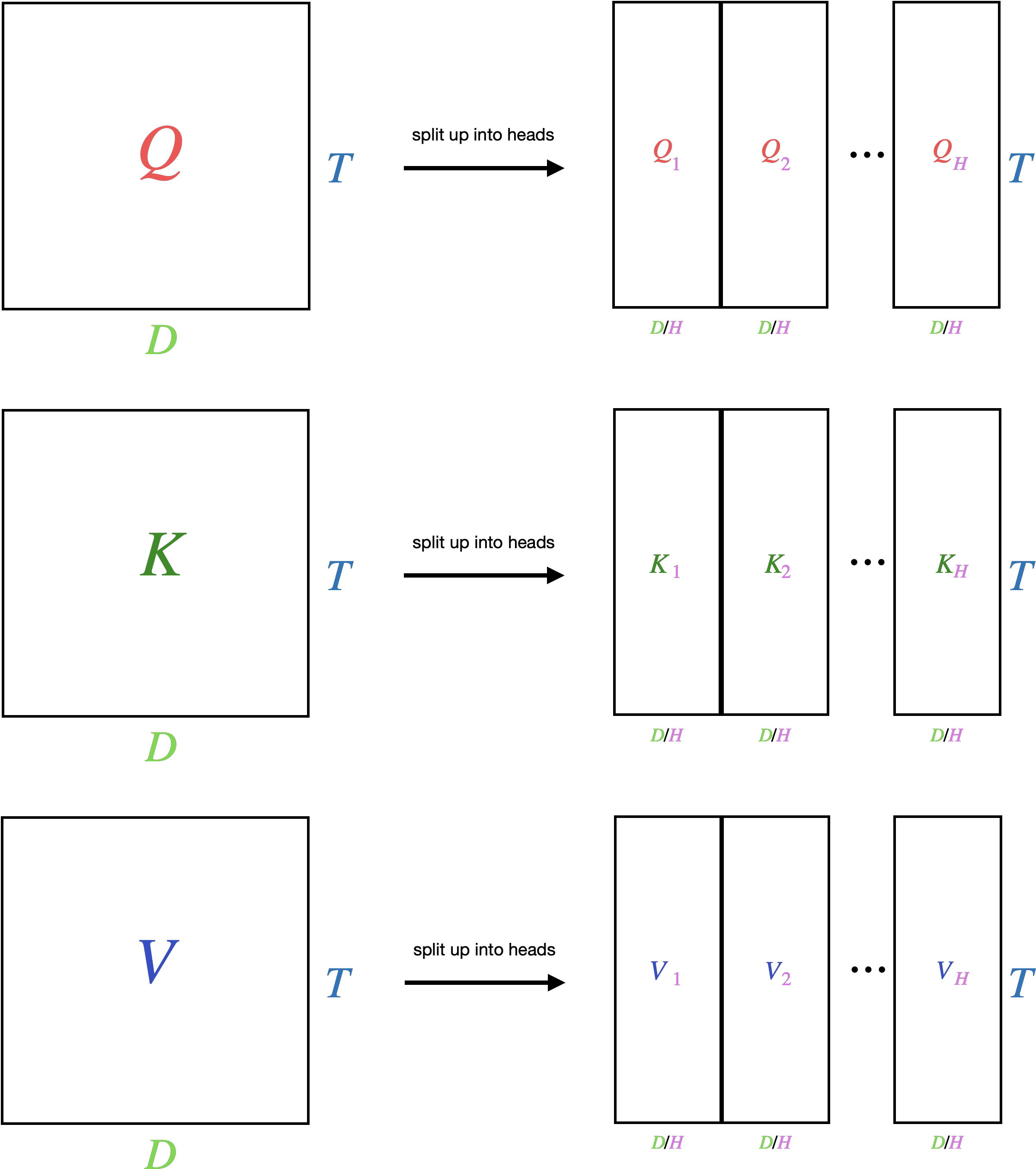
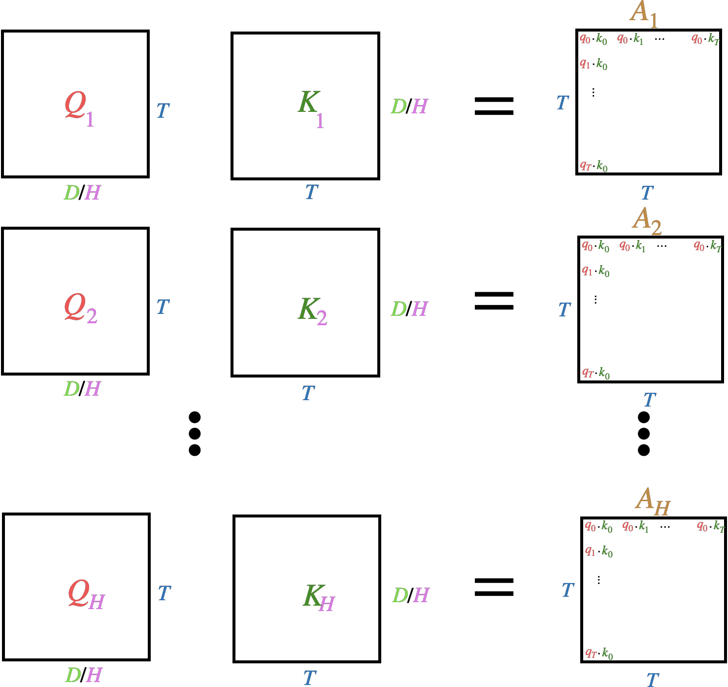
multi-headed attention — Figure 11: Multi-headed attention Q,K,V

Now we take each $H$ $Q$ and $K$ tensors and compute $A_h$ for each head. This results in $H$ $T \times T$ attention weight tensors, instead of the 1 we had previously. This increases the memory requirements by a factor of $H$. This allows the model to learn $H$ different measures of similarity between each token.

multi-headed attention weights — Figure 12: Multi-headed attention weights

Finally, we weight each of the $H$ value tensors $V$ using the $H$ attention weight tensors. This results in $H$ $T \times D/H$ tensors which get stacked together as a single $T \times D$ tensor, the same dimensionality as in the single-headed scenario.

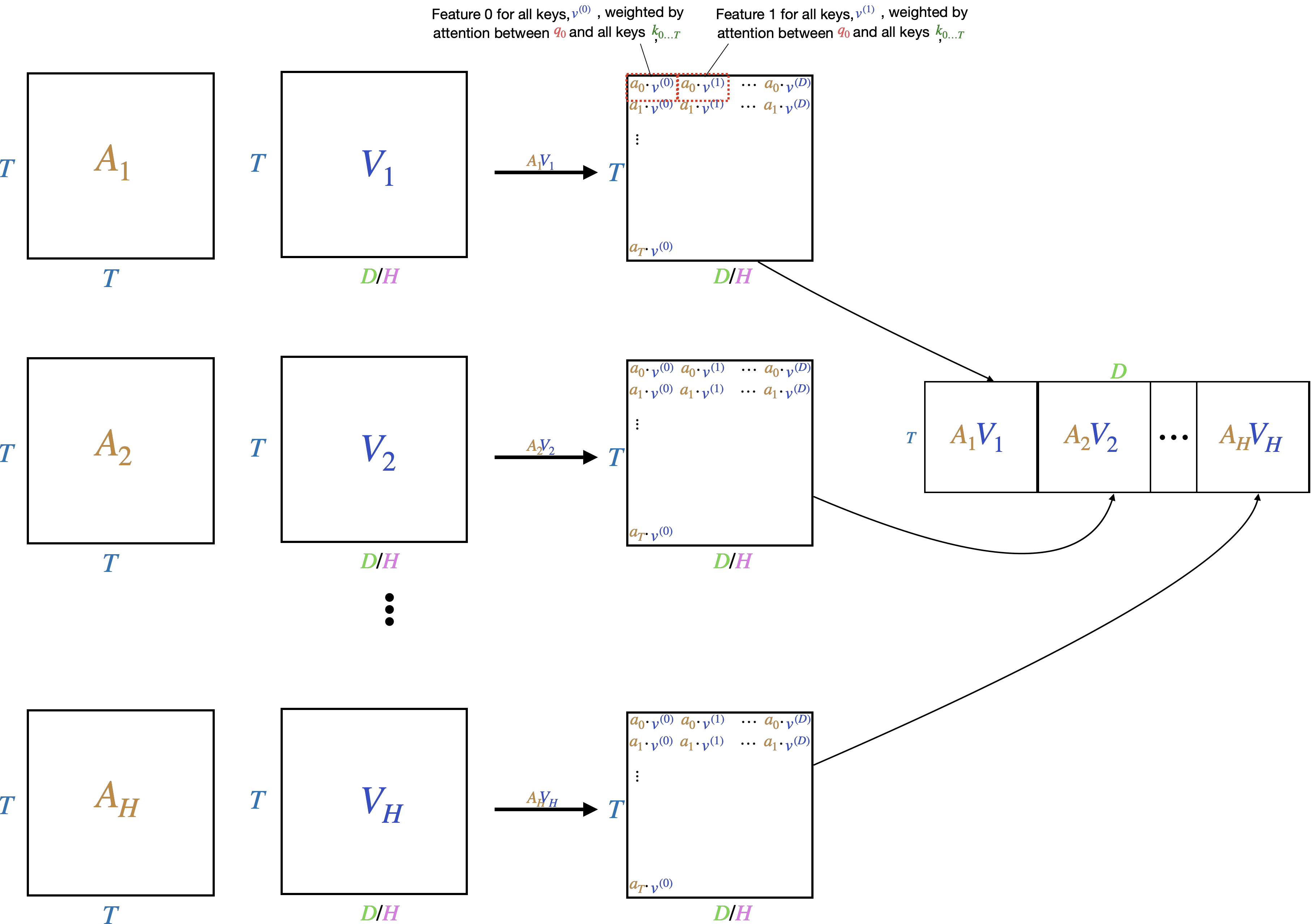
multi-headed feature vectors — Figure 13: Multi-headed weighted feature vectors

The stacked multi-headed attention output is on the right.

For the cost of $H$ attention weight tensors instead of 1, the model is able to learn $H$ different queries, keys, values, and similarity measures.

code example

step 1.

In code, using pytorch, if we have a (T, D) tensor for Q, K, and V respectively, we can split up into $H$ different heads using a tensor view

Q = Q.view(T, H, D//H).transpose(0, 1)
K = K.view(T, H, D//H).transpose(0, 1)
V = V.view(T, H, D//H).transpose(0, 1)

This will produce a tensor of size (T, H, D//H). We swap T and H so that H becomes the batch dimension, which will be needed in the next step, resulting in a (H, T, D//H) tensor.

step 2.

To calculate $H$ $T \times T$ attention tensors,

A = Q @ K.transpose(-2, -1) * (1.0 / math.sqrt(K.size(-1)))

Note that in pytorch if we use @ which is the overloaded symbol for matmul, that if we have a (..., A, B) dimensional tensor multiplied with (..., B, A) tensor, then the ... dimensions are used as a batch dimension and the remaining dimensions are multiplied as in the typical 2d case. Here H is the batch dimension, but this would usually be part of a mini-batch in which case B, H would be the batch dimension. This gives us H (T, T) tensors, which are calculated in parallel.

We map the attention weights for each query to a probability distribution using softmax

A = F.softmax(att, dim=-1)

step 3.

Finally, we obtain the weighted feature vectors:

y = A @ V

This uses the same batch matmul procedure as in the attention calculation. We are multiplying (H, T, T) tensor with (H, T, D/H) so this produces a (H, T, D/H) tensor.

We stack the H weighted feature tensors together

y = y.transpose(1, 2).contiguous().view(T, D)

which produces the final (T, D) tensor.

Note:

There is an even more optimized code path to calculate all this using torch.nn.functional.scaled_dot_product_attention which uses optimized cuda kernels shown to be much faster and with less memory footprint than the above naive implementation

decoder

So far we’ve been looking at the left-side of the transformer diagram, at the encoder. The decoder plays a similar role to the decoder in the encoder-decoder RNN—it decodes the learned representation from the encoder into a sequence. Like the RNN decoder, the transformer decoder will output a single token at each timestep ${1 \ldots T}$ iteratively. It is similar in many ways to the encoder. It will use self-attention to attend to the tokens it has output and will output a $d$-dimensional vector at each timestep. Unlike the encoder:

We don’t want the decoder to see into the future during training. This is accomplished using masked attention
We want the decoder to also attend to the encoder outputs. This is known as cross-attention

masked attention

Let’s take a look at the Masked
Multi-Head
Attention box in the Transformer architecture diagram. In the RNN decoder, we don’t peek into the future by its nature, since we process each token sequentially. This is the so-called “autoregressive” modeling. We need to be careful that the transformer decoder doesn’t see into the future during training, since the self-attention mechanism is able to look at all tokens, including future tokens. In other words, in the target sequence [I, have, a, cat], we do not want I to “know about” have a cat. This is because we do not know what the correct output is when this is used on novel input sequences, and letting the model see into the future would make it incapable of generating novel correct sequences. How are we going to accomplish this?

The self-attention mechanism allows every query $q_{1 \ldots T}$ to attend to every key $k_{1 \ldots T}$. But we only want query $q_t$ to attend to keys $k_{1 \ldots t-1}$.

To accomplish this, we can zero out attention weights for keys $k_{t \ldots T}$. That way when we compute the softmax over each key, these keys won’t contribute.

The trick, in code, is to set the attention output $AV$ to $-\inf$ using an upper triangular matrix for all $k_{t_k>=t_q}$ where $t_k$ is the key timestep and $t_q$ is the query timestep. The attention masking is commonly referred to as causal mask.

causal_mask = torch.triu(torch.ones(t_q, t_k))
causal_mask = causal_mask.masked_fill(causal_mask.bool(), -float('inf'))
att = (q @ k.transpose(-2, -1)) * (1.0 / math.sqrt(k.size(-1)))
att += causal_mask
att = F.softmax(att, dim=-1)

Example:

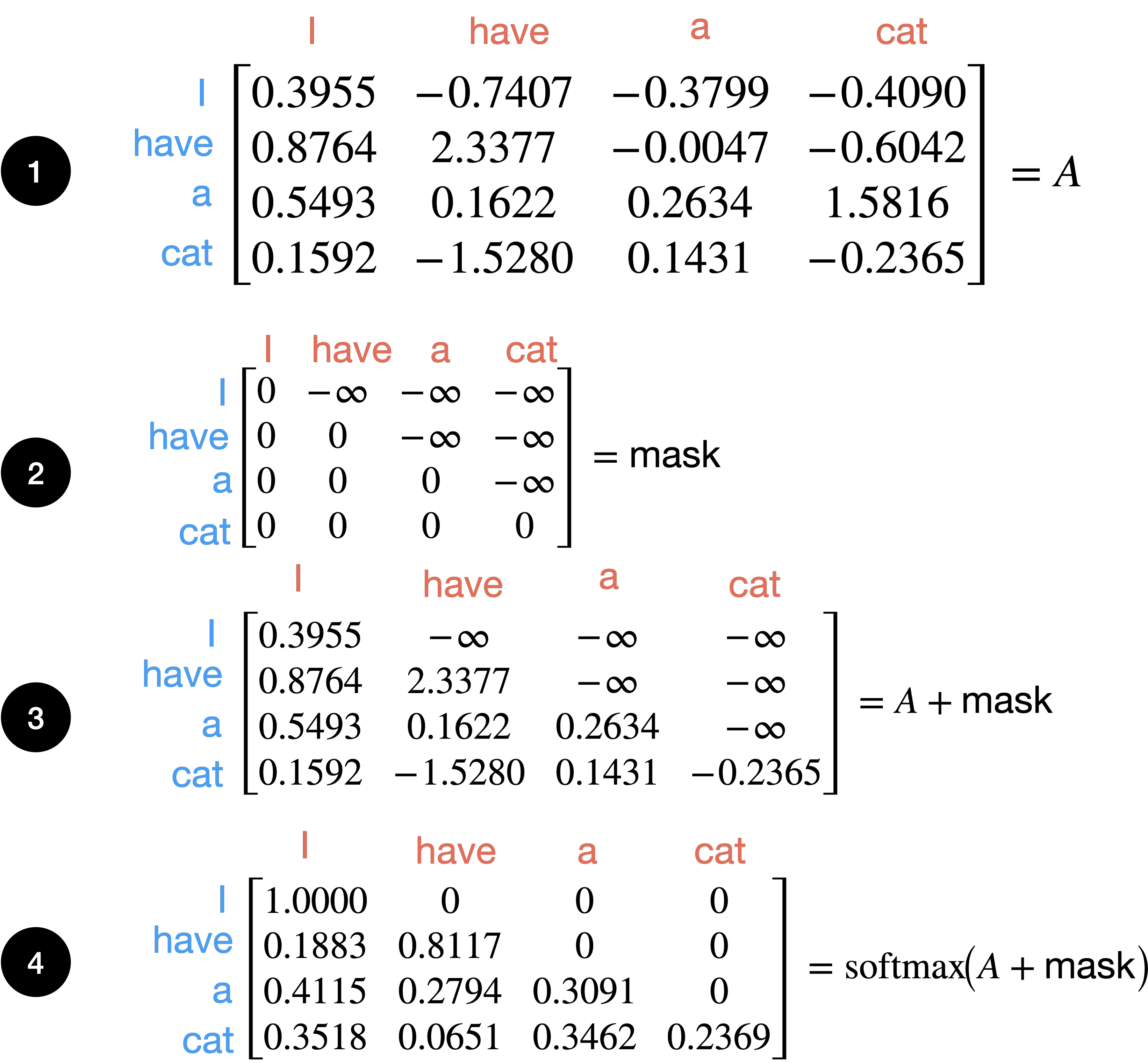
masked self-attention — Figure 14: Masked self-attention

In step 1 we initialize $A$ to hypothetical values where queries are in blue and keys in red. In step 2 we initialize our upper triangular matrix $\text{mask}$ to have the value $-\inf$ in the nonzero slots, and is the same size as $A$. In step 3 we add $\text{mask}$ to $A$. In step 4 we take the $\text{softmax}$ across columns for each row. Note the effect of the mask. For the first token I all other timesteps are zeroed out. For the second token, have it is able to attend to itself and the previous token I. For the third token a, it is able to attend to itself and I, have, but not to the next token cat, etc.

cross attention

Using masked self-attention, the decoder can pay attention to the tokens in the target sequence. However, we also need the decoder to pay attention to the encoder’s representation of the source sequence. To do this, we’ll use the concept of cross-attention which is the Multi-Head
Attention box in the decoder (right half) of the Transformer architecture diagram.

Using self-attention, a sequence can pay attention to itself. However, we can also use attention so that a sequence $A$ can pay attention to another sequence $B$. We’ll use that so that the decoder can pay attention to the encoder’s representation.

Let the source sequence be [J'ai, un, chat] and the target sequence be [I, have, a, cat].

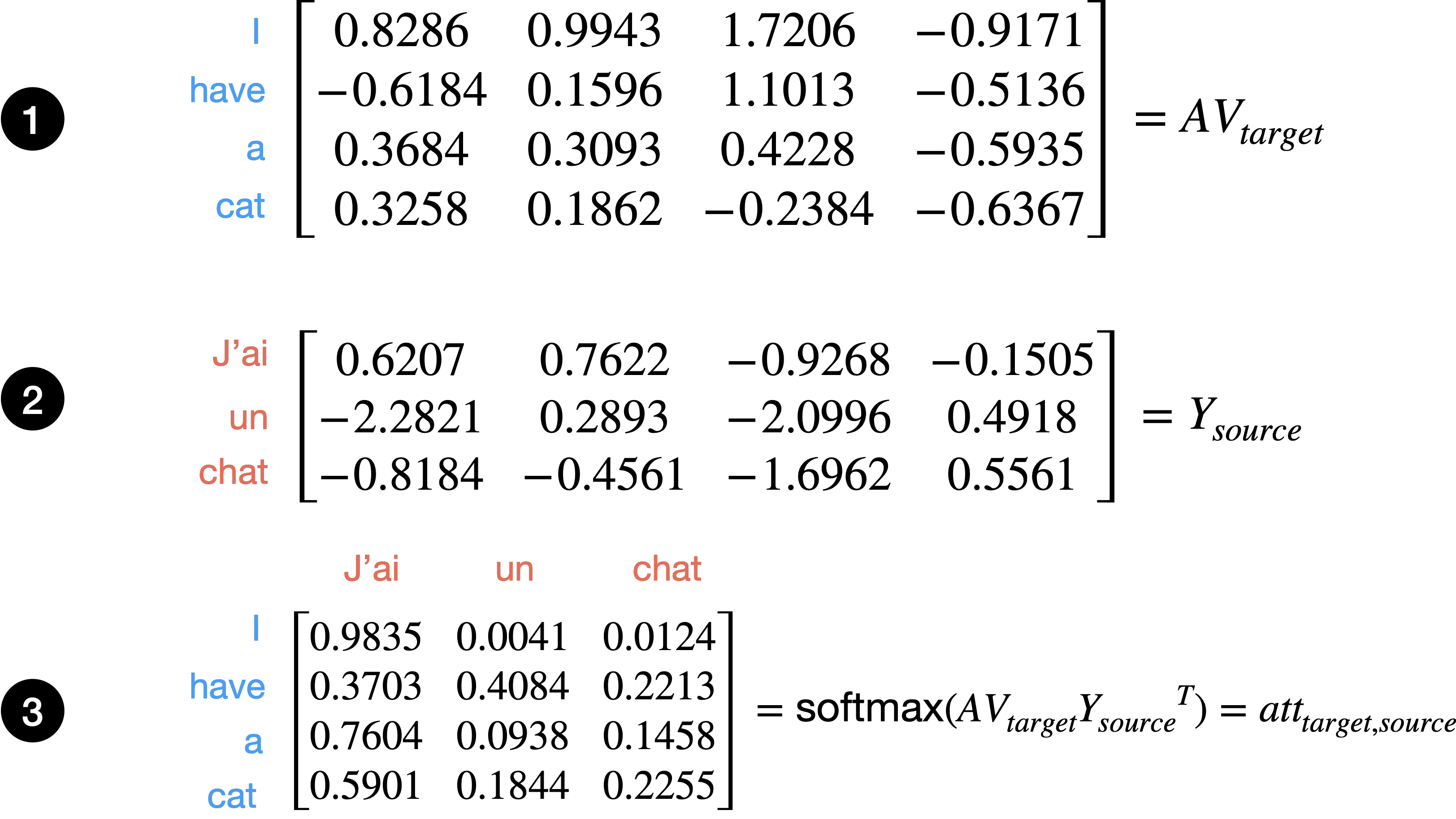
cross attention — Figure 15: Cross attention example

In this example, 1 let $AV_{target}$ be $AV$ for the target sequence and 2 let $Y_{source}$ be the output from the encoder for the source sequence. Again, let denote a value for a query and denote a value for a key. Then in 3 we compute attention weights between the queries from the target to the keys in the source. This is a hypothetical example, but $att_{target,source}$ is saying that “I” attends most strongly to “Jai,” “have” to “un,” etc.

This shows how the target sequence can attend to the source sequence, crucial for translation in which we need to know how the target translation aligns with the source sequence.

Other components of the transformer

There are a few other components to the transformer. We’ll cover Feed Forward , positional encoding, Add & Norm , Linear , and Softmax next.

Feed forward network

Recall that the output of the attention mechanism is $AV \in \mathbb{R}^{T \times D}$. At this point there is no nonlinearity, and so the model is limited in its representational capacity. We add a position-wise feed forward network with a single hidden layer, where $x$ the attention output.

\[\begin{aligned} \mathrm{FFN}(x) &= W_2\bigl(\sigma\bigl(W_1\,x + b_1\bigr)\bigr) + b_2, \\[6pt] W_1 &\in \mathbb{R}^{H\times D}, \quad W_2 \in \mathbb{R}^{D\times H}, \\[6pt] \sigma(\cdot) &: \quad (\text{activation function, e.g., ReLU or GELU}) \end{aligned}\]

This whole sequence $AV$ followed by $\mathrm{FFN}$ is repeated $N_x$ times, where the sequence is considered a “block” and the output of ${block}_l$ becomes the input of ${block}_{l+1}$, in other words the model starts attending to its own feature representations.

positional encoding

The attention mechanism treats each token independently. In other words, it does not care or no about order. This is known as a “bag of words” model because it’s as if the words were put in a bag and mixed up. This is a problem because the sentences “this is a bad bagel” and “is this a bad bagel” would be identical. Let’s take a look at an example.

As we can see, when we did not use positional encoding the attention output y_perm is permuted in the same way as the input x_perm. Therefore, both orderings would be treated the same by the model.

However, when we add a positional encoding by adding positional_embedding to x, then order matters since when we shuffle x, now the positional_embedding indicates the order and y_with_pos and y_shuffle_with_pos are different.

The positional_embedding is just a learned embedding lookup for each token position. One concern is that the positional embedding must be learned and might not be well-trained for token positions that fall outside the normal range (e.g., unusually long sequences). (Vaswani et al., 2017) use a non-learned sinusoidal function to add positional information instead, but they didn’t notice any performance difference between the sinusoidal function vs. the positional embedding. Future models such as GPT-2 use positional embedding.

Next, we’ll cover Add & Norm , which is two steps: layer normalization and residual connections.

layer norm

For certain types of models, including CNNs, batch normalization (Ioffe & Szegedy, 2015) is typically used to stabilize the network, and this has been shown to decrease the number of iterations it takes a deep model to converge. Discussion about normalization techniques is outside the scope of this article, but I wanted to motivate why a different normalization technique is used for transformers than was previously used.

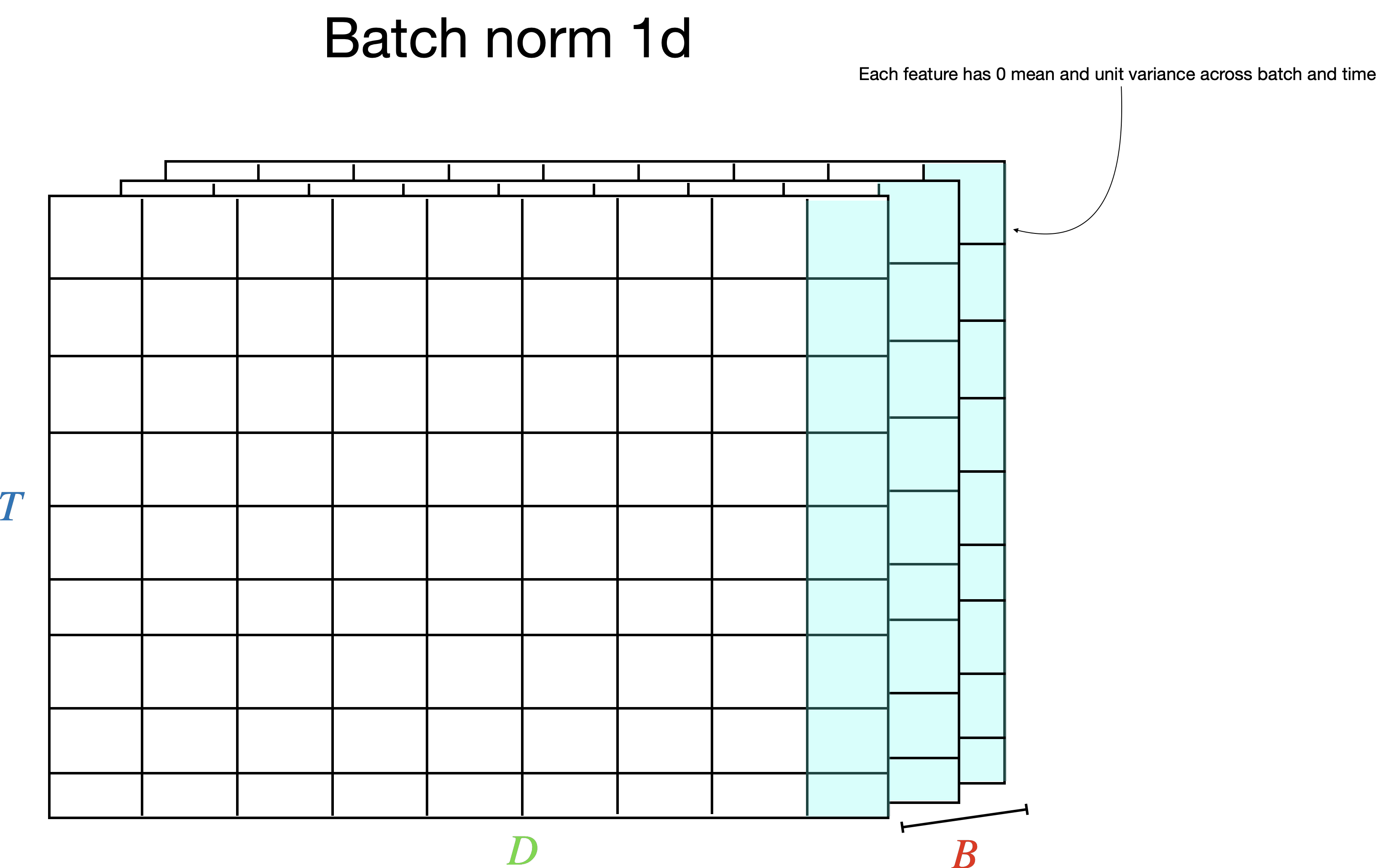
If we were to apply batch normalization in one dimension for sequential text data where the shape is (B, T, D), the normalization is applied for each feature over each (B, T), yielding a D-dimension $\mu$ and $\sigma^2$ vector, containing the statistics for each feature over batch and time, as well as D-dimensional $\gamma$ and $\beta$ to scale and shift the distribution. Normalization is applied over the batch and time dimension:

\[\mu_d \;=\; \frac{1}{B\,T} \sum_{b=1}^{B}\sum_{t=1}^{T} x_{b,t,d} \qquad \sigma_d^2 \;=\; \frac{1}{B\,T} \sum_{b=1}^{B}\sum_{t=1}^{T} \bigl(x_{b,t,d}-\mu_d\bigr)^{2} \qquad \hat x_{b,t,d} \;=\; \frac{x_{b,t,d}-\mu_d}{\sqrt{\sigma_d^2}} \qquad y_{b,t,d} \;=\; \gamma_d\,\hat x_{b,t,d} + \beta_d\]

This is a problem for sequential text data for several reasons.

Each token’s features represent different things, and it’s not natural to normalize over the features of different tokens.
This cannot be used when sequences are of different lengths, since in that case the sequences are padded to the longest sequence in the mini-batch, and we don’t want to include padding features when computing statistics. We would have to mask this out somehow.
At inference time when we decode the sequence sequentially, we’d be using running statistics that were calculated based on an entire sequence.

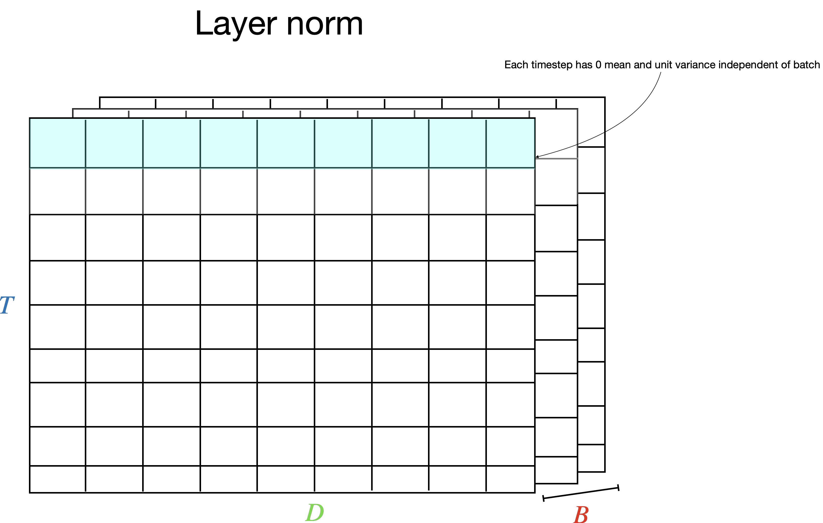
For sequential text data, instead, we’d like to normalize each timestep individually, without the features from other timesteps being included. This is what (Ba et al., 2016) does. Instead of normalizing along the batch and time dimension as in BatchNorm1d, layer norm normalizes along each feature axis $D$ for each timestep, resulting in a D-dimension $\mu$ and $\sigma^2$ vector, containing the statistics for each feature as well as D-dimensional $\gamma$ and $\beta$ to scale and shift the distribution, for each timestep. Every timestep in the batch is normalized individually:

\[\mu_{b,t} \;=\; \frac{1}{D} \sum_{d=1}^{D} x_{b, t,d} \qquad \sigma_{b,t}^2 \;=\; \frac{1}{D} \sum_{d=1}^{D} \bigl(x_{b, t,d}-\mu_{b,t}\bigr)^{2} \qquad \hat x_{b,t,d} \;=\; \frac{x_{b,t,d}-\mu_{b,t}}{\sqrt{\sigma_{b,t}^2 + \varepsilon}} \qquad y_{b,t,d} \;=\; \gamma_d\,\hat x_{b,t,d} + \beta_d\]

Now we can normalize over each token individually, and so:

Layer norm normalizes over each timestep individually, instead of including information from other timesteps.
We can handle sequences of arbitrary lengths since we normalize each timestep individually.
We don’t need to track running statistics, since each timestep is normalized on the fly.

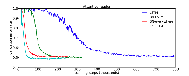
We can also see that experimentally, layer norm gives faster convergence for sequential text data, where in this case layer norm is used in a multimodal model to model images and captions:

residual connections

Residual connections (aka skip connections) allow information to flow through the network. (He et al., 2016) observed that increasing the size of the network leads to worse training performance, which did not make sense, since deeper networks should be able to fit strictly more complex functions than shallower networks. He et al. observed this was because the signal was getting “lost.” Let’s look at a basic example.

Consider $y_1 = f_1(x)$ where $f_1$, which is a blackbox function, and $y_2 = f_2(y_1)$ which takes as input $y_1$.

We want to compute $\frac{\partial y_2}{\partial x}$, i.e., how does an inner input affect the output, which is $\frac{\partial y_2}{\partial x} = \frac{\partial f_2}{\partial y_1}\frac{\partial y_1}{\partial x}$ due to the chain rule.

If the upstream gradient $\frac{\partial f_2}{\partial y_1}$ is $<< 1$ or 0, then $\frac{\partial y_2}{\partial x}$ will be diluted or 0.

Residual connections are beautifully simple but powerful. If instead of computing $y_2 = f_2(y_1)$, we compute $y_2 = y_1 + f_2(y_1)$, then

\[\begin{align*} \frac{\partial y_2}{\partial x} &= (1 + \frac{\partial f_2}{\partial y_1})\frac{\partial y_1}{\partial x} \\ &= \frac{\partial y_1}{\partial x} + \frac{\partial f_2}{\partial y_1}\frac{\partial y_1}{\partial x} \end{align*}\]

Notice that just by adding the input $y_1$, we have made sure that the inner gradient is propagated without being diluted/zeroed out by the upstream gradient.

Why are they called “residual” connections? Because now if the downstream layer $f_2$ contributes meaningfully to the signal, then the term $\frac{\partial f_2}{\partial y_1}\frac{\partial y_1}{\partial x}$ gets added to the gradient $\frac{\partial y_1}{\partial x}$; otherwise we still propagate the inner term $\frac{\partial y_1}{\partial x}$ which tells us how the input affected an earlier layer in the network.

In the transformer we use residual connections in the following way:

def forward(x):
    x = x + self.multi_head_attention(x)
    x = self.layer_norm[0](x)
    x = x + self.mlp(x)
    x = self.layer_norm[1](x)
    return x

The input x is added to the output in order to propagate the gradient of the input. Notice that the gradient must flow through the layer norm. (Xiong et al., 2020) studied if it is better to allow the gradient of the input to flow without it being modified by the layer norm. The original transformer “between residual block” layer norm is referred to as “post-layer normalization,” while the approach by Xiong et al. is “pre-layer normalization.”

In code the pre-layer normalization looks like

def forward(x):
    x = x + self.multi_head_attention(self.layer_norm[0](x))
    x = x + self.mlp(self.layer_norm[1](x))
    return x

(Xiong et al., 2020) found that placing the layer norm within the residual blocks allows for a faster convergence than if the layer norm is placed between the residual blocks. This is because when the layer norm is placed between the residual blocks, then the training requires a learning rate warmup to achieve good results. Without the warmup, training converges more quickly, and (Xiong et al., 2020) shows that learning rate warmup is not needed if we place the layer norm inside the residual blocks. The former approach is called post-layer normalization transformer while the latter is pre-layer normalization transformer.

They have a nice picture showing this:

pre vs post ln — Figure 19: Pre vs post layer norm. Figure from (Xiong et al., 2020).

Notice that compared to post-layer norm, here the gradient of x flows through without the gradient being modified by the layer norm. This is what yields faster convergence without learning rate warmup.

(Xiong et al., 2020) showed this experimentally, where we can see clearly that the pre-layer norm without warmup converges faster than the post-layer norm with warmup:

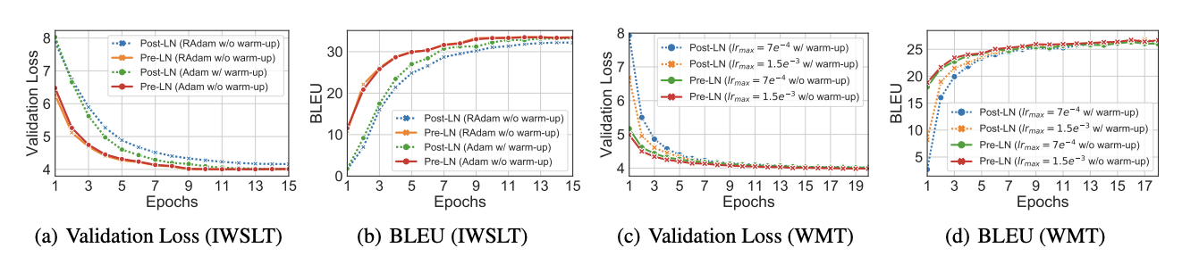
Because of this, transformer architectures such as GPT adopted pre-layer norm (although with warmup, go figure)

Putting it all together

We want the decoder to predict the next token $y_{t+1}$ at each timestep $t$. To do this, we shift each token 1 unit to the right and fill the token at $t=0$ with a start of sequence token. The target sequence [I, have, a, cat] becomes [<sos>, I, have, a, cat] so that $y_0$ is <sos>, $y_1$ is I, etc.

We feed the source sequence through the encoder, which produces an encoded representation, and the shifted target sequence through the decoder, which also makes use of the encoded representation of the source sequence using cross-attention. The output of this is a $T \times D$ tensor. But we are not quite done. We need to learn to predict the target sequence from the source sequence. The $T \times D$ tensor output by the decoder needs to be mapped to $T \times C$ where $C$ is the number of tokens in the vocabulary, and for that we’ll use a $D \times C$ fully connected layer at the end, which is indicated by the Linear box in the Transformer architecture diagram. Recall that the token embedding lookup maps $C$ tokens to $D$-dimensional vectors. Because the final fully connected layer can be thought of as the opposite, mapping $D$ to $C$ instead of $C$ to $D$, we can reuse the weights from the embedding lookup. This saves a lot of extra parameters since $D$ and $C$ can be quite large. The logits from the fully connected layer are run through the Softmax function to produce a probability distribution over tokens. We then backpropagate using cross-entropy over the $C$ categories as the loss function.

During inference, we will iteratively decode a single token at a time since we do not have a target sequence. After every iteration, we’ll add the decoded token to the decoded sequence to generate the translated sequence, and we’ll stop once we’ve predicted the end-of-sequence token or hit a maximum number of iterations.

Experiments and results

I implemented a transformer using the approach described in Vaswani et al., to reproduce results, and trained on the WMT ‘14 train set and tested on the WMT ‘14 test set. I was interested in reproducing results in the paper but also wanted to see how the runtime and performance of the model compares to the RNN. Why is the transformer considered a breakthrough? Transformers allow better parallelization than RNNs since we do not need to iterate through each token to process a sequence as in an RNN, but can instead process the entire sequence in parallel using tensor multiplication. So this ought to be more efficient, but how much more efficient? This efficiency, I think, is what enables transformers to perform much better than RNNs at scale since we can train on much larger datasets and models more quickly, and I think this is what allowed researchers to test the hypothesis of whether LLMs would “wake up” when the model size + data size increased. Without transformers, I don’t think we would have reached this paradigm shift.

My primary interest was in reproducing the results reported in Vaswani et al.

My secondary interest was in seeing how the transformer performance in terms of accuracy as well as runtime and scalability compares to the RNN performance.

Lastly, the transformer architecture uses an encoder-decoder architecture; however, GPT and other LLMs use a decoder-only architecture. They use a decoder-only architecture since they train in a different self-supervised regime where they take a large amount of text and just try to predict the next token. This is different from the translation problem in which we want to take a sequence and predict an entire sequence correctly. But I was motivated to try using a decoder-only model for the problem of translation since a decoder-only model is simpler than an encoder-decoder. It also seems easy to frame the translation as predicting the next token rather than encoding the source sequence and then producing the translation.

Dataset

See the previous post

Model

The model hyperparameters are the same as Transformer base in Vaswani et al.

\[\begin{array}{|c|c|c|c|c|c|} \hline d_{\text{model}} & h & P_{drop} & d_{ff} & N & \epsilon_{ls} \\ \hline 512 & 8 & 0.1 & 2048 & 6 & 0.1 \\ \hline \end{array}\]

where

$d_{model}$ is the hidden dim in every layer of the model
$h$ is the number of attention heads, and so the hidden dim in every head is $512/8=64$
$P_{drop}$ is the dropout
$d_{ff}$ is the feedforward hidden dim
$N$ is the number of blocks
$\epsilon_{ls}$ is the label smoothing strength

A difference between my model and the transformer base model is that I used a separate vocabulary and embedding lookup for both the encoder and decoder, since that was the approach I followed for the RNN model. I used a vocab size of $30,000$ for both the source and target languages, compared to a vocab size of $32,000$ total vocabulary size used by Vaswani et al.

The model had $74M$ parameters compared to $65M$ in transformer base, with the difference stemming from the $60,000$ embedding vectors compared to $32,000$.

Training

Byte-pair encoding was used for tokenization. See the previous post for details.
Data was split randomly into train/val using 99.9% of the data for train (4000 val examples)
I used 3 nvidia V100 GPUs for 24 hours with a batch size of 128 (228,000 iterations).
Cross-entropy loss was used, and the model’s weights were updated if the cross-entropy loss decreased.
Training was done using float16 mixed precision using automatic mixed precision provided by pytorch (torch.amp)
$\text{AdamW}$ optimizer using cosine annealing with warmup learning rate scheduler was used. Warmup number of steps is $2000$, min learning rate is $6e^-5$, and the max learning rate is $6e^-4$

Results and discussion

The reproduced model achieves equivalent test-set performance as Transformer base. FLOPs calculation is using $$C = 6ND$$ per Kaplan et al. 2020.
Model	Non-embedding Parameters	FLOPs	BLEU
Transformer Base	65M	$$1.95 \times 10^{18}$$	38.1
This model	60M	$$1.57 \times 10^{18}$$	38.6

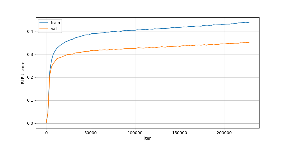
The test set performance shows that we were able to achieve the same performance.

From the plot of train/validation BLEU score, we can see that the model did not converge and could have continued training with increased performance.

Attention examples

Let’s look at the encoder self-attention, and decoder-cross attention calculated by the model. I’m skipping decoder self-attention as I don’t speak French, and it is most likely similar in nature to the encoder self-attention. I’ve chosen the same running example from the test set “But why such optimism for some and pessimism for others?” → “Les raisons d’un tel optimisme, chez les uns, et pessimisme, chez les autres ?”.

Encoder self-attention

I’ve broken down the self-attention by layer which can be toggled by the slider at the bottom, and each subplot is a single head of attention. The query tokens are on the left and key tokens on the right. The line weight indicates the attention weight ranging from $[0, 1]$.

Here’s what I notice, focusing on a couple layers for brevity:

Layer 1
- In layer 1 the attention seems pretty diffuse where each token in general seems to be attending to every other token
Layer 2
- In layer 2 we start to see more specialized heads. In head 2 token $j$ is attending to the previous token $j-1$, and in head 4 token $j$ attends to the next token $j+1$.
- Interestingly, many of the tokens are attending to the end of sequence token </s>.
Layer 6
- Head 7 ? attends to why
- Head 8 token $j$ attends to itself
- Head 6 some tokens attend to another instance of itself elsewhere in the sequence, e.g., the first for attends to the 2nd for, or if no other instance is in the sequence, then it attends to itself

As we can see, the heads are performing different functions in terms of learning the structure of the sequence.

Decoder cross-attention

The following example is generated by collecting attention weights from the decoder during inference generation of the sequence.

A few observations:

Throughout all layers a significant amount of attention is given to the end of sequence token </s>, particularly in early layers 1-3
Some heads, e.g., head 7 in layer 3 align output tokens with the corresponding input token (Mais -> But, porquois -> why, etc). This makes sense and what I would expect the model to do for translation, since the output needs to be aligned with the input.
Other heads, e.g., head 1 in layer 5 align output tokens with the corresponding input token that follows it (in the phrase “Mais porquois” (But why), “Mais” (but) attends to why,” etc.)

Many of these observations on attention behaviors are not unique to this data/model but are found in other research and LLMs, such as in (Clark et al., 2019) in which they also find that a significant amount of attention weight is placed on [SEP], the token used to indicate a sequence boundary (similar to </s> that I used). They argue that this is a “no-op” or a sort of fallback behavior. They also find that many heads do simple and similar things such as just attending to the previous or the next token.

Contrary to what the paper observes, heads in the same layer don’t always perform the same function, e.g., head 2 and 4 in layer 2 of the encoder self-attention clearly perform previous token and next token alignment respectively.

Transformer vs RNN architecture

One of the motivating reasons for studying the transformer was to try to understand the benefits it has over the RNN. We know that researchers and AI companies have adopted the transformer architecture for LLMs, and so we’d like to try to understand why LLMs weren’t built with a different architecture, such as the RNN.

Here is a summary table comparing RNN with Transformer efficiency and performance.

Model	Parameter count¹	Num. tokens processed²	Num. GPU hours³	GPU	FLOPs⁴	FLOP/s	BLEU⁵
RNN	158M	6.1 B	159	nvidia V100	$5.78 \times 10^{18}$	$1 \times 10^{13}$	.30
Transformer	60M	4.37 B	30	nvidia V100	$1.57 \times 10^{18}$	$1.45 \times 10^{13}$	.38

runtime efficiency

First, which model ran faster? The RNN must process each token sequentially, while the transformer can process all tokens in parallel using matrix multiplications, and so we would expect the transformer to make better use of the hardware. Deep learning model’s runtime complexity is typically measured in terms of FLOPs (floating point operations), rather than using big-O notation as is typical for algorithms. Neural networks essentially do many adds and multiplies. A single add and a single multiply would count as 2 FLOPs. A matrix multiply $AB$ where $A$ is $[M, N]$ and $B$ is $[N, P]$ would require $2*M*N*P$ FLOPs. If $A$ is $[49, 1]$ and $B$ is $[1, 10000]$ then there are $980,000$ FLOPs. Models that require more FLOPs are computationally more expensive.

How are FLOPs calculated? In (Vaswani et al., 2017) they calculate FLOPs

by multiplying the training time, the number of GPUs used, and an estimate of the sustained single-precision floating-point capacity of each GPU

This relies on the floating point capacity of the GPU and assumes 100% or near 100% saturation of the GPU and is GPU-dependent. If the model doesn’t 100% saturate the GPU, then this calculation will be an overestimate.

Later work (Kaplan et al., 2020) derived that for most neural network models the number of FLOPs can be calculated as $C=6ND$ where N is the number of parameters in the model and D is the number of inputs (see this blog post for an explanation). Using this method to estimate the number of FLOPs, the transformer performed $1.57 \times 10^{18}$ of FLOPs while the RNN performed $5.78 \times 10^{18}$ FLOPs. The transformer trained for 30 GPU hours and performed $1.45 \times 10^{13}$ FLOP/s while the RNN trained for 159 GPU hours and performed $1 \times 10^{13}$ FLOP/s, so the transformer was able to run 1.45x faster than the RNN.

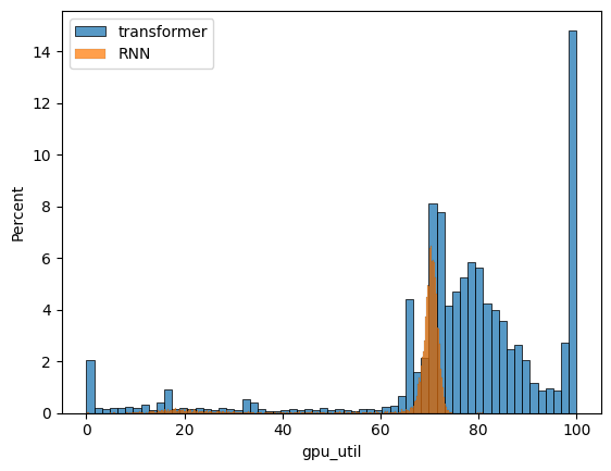
This is also supported by looking at GPU utilization logs. Since the transformer keeps the GPU busier by processing tokens in parallel, it is able to run more operations / second.

Translation quality

Recall that the RNN achieved 30 WMT’14 test set BLEU, while the transformer achieved 38 BLEU and so the transformer had better translation quality. It also did this with less data and with fewer weights. The RNN was trained on 6.1B tokens and contained 158M params, while the transformer only trained on 4.7B tokens and contained 60M params.

So the transformer achieved significantly better translation quality using fewer parameters and 25% less data, and was 1.45x more efficient in terms of theoretical FLOP/s.

Encoder-decoder vs decoder-only

The transformer architecture used by LLMs is largely the same as in the original transformer but with a few differences. The differences include:

GELU activation function (Hendrycks & Gimpel, 2016) instead of ReLU
layer norm within the residual block (pre-LN)
additional layer norm before the final linear layer
Decoder-only (no encoder)

The first three are fairly simple architectural details that yield an improvement. The last difference, decoder-only vs. encoder-decoder, requires some explanation. In the original transformer paper, the transformer includes both an encoder and a decoder. The encoder encodes the source text while the decoder produces the output. This makes sense since there is a finite input (the input text) that must be understood to produce the output. However, LLM pretraining works by taking in a context of text and predicting the next token. This is what the decoder does in our encoder-decoder model. It takes as context the currently predicted sequence and predicts the next token. What if instead of just taking the target text or predicted text as context, it also prepended the source text? Then we can treat the entire source + target/predicted text as a single sequence and learn to predict the next token.

I largely followed (Wang et al., 2021) which had the same idea.

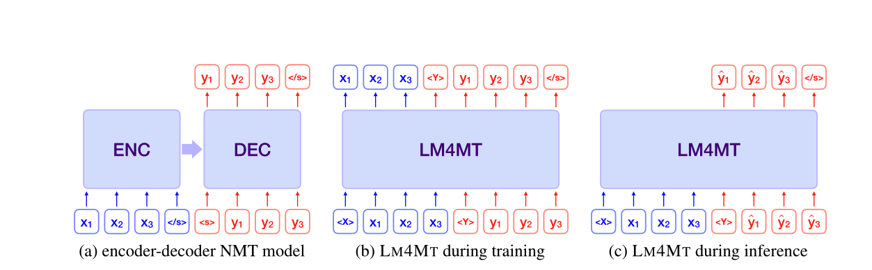
lm4mt — Figure 26: Decoder-only model. Diagram from (Wang et al., 2021). During training, the source and target texts are concatenated into a long sequence and the next token is predicted. During inference the source text is given as input, and the predicted text is concatenated to it.

As an example, if the following are the source and target texts, respectively, they would get concatenated into a single long input:

concatenated input: <source> Macedonian entrepreneurs and their descendants eventually employed their numerical strength within the food service industry as a catapult into a variety of larger and more sophisticated ventures. <target> Finalement, des entrepreneurs macédoniens et leurs descendants utiliseront la force du nombre dans l’industrie du service alimentaire comme un tremplin vers différentes entreprises plus perfectionnées et plus importantes.

You’ll notice that the source and target texts are separated by a special language tag token, which (Wang et al., 2021) found to be beneficial.

One concern is that the goal, remember, is to translate text. We want our measure of success to be how well the output aligns with the expected output. However, if we were to model the concatenated text next token prediction using cross-entropy loss, then we would also be tuning the model to predict the next token in the source text as well as the target text. We don’t care how well the model can predict the next token for the source text, but we do for the target text.

For this reason (Wang et al., 2021) separated the loss into a multi-task loss with two parts. Recall that in the encoder-decoder, the loss is only measured on the target sequence as the cross-entropy loss

\[\mathcal{L}_{CE} = -\sum_{1}^{T}\text{log}P\bigl(y_t \mid \mathbf{x}, \mathbf{y}_{<t}\bigr)\]

. However, in the decoder-only setting, the source and target are concatenated. (Wang et al., 2021) break up the loss into 2 parts: $\mathcal{L}^{AE}$, the autoencoder loss which is defined as

\[\mathcal{L}^{AE} = -\sum_{1}^{S}\text{log}P\bigl(x_s \mid \mathbf{x}_{<s}\bigr)\]

and the machine translation loss $\mathcal{L}^{MT}$ which is defined as

\[\mathcal{L}^{MT} = -\sum_{1}^{T}\text{log}P\bigl(y_t \mid \mathbf{x}, \mathbf{y}_{<t}\bigr)\]

where $S$ is the number of tokens in the source sequence, $T$ is the number of tokens in the target sequence, $\mathbf{x}$ is the source sequence, and $\mathbf{y}$ is the target sequence.

The total loss $\mathcal{L}$ is therefore

\[\mathcal{L} = \mathcal{L}^{AE} + \mathcal{L}^{MT}\]

This loss differs from the transformer loss $\mathcal{L}_{CE}$ in that we’re computing loss on the source sequence as well as the target sequence.

Since we’ve separated the loss into two parts, 1 for the source sequence and another for the target sequence, we can control each separately. Since the goal is translation, we might want to focus more on the $\mathcal{L}^{MT}$ component at later stages in training. This is what (Wang et al., 2021) did, they added a term $\lambda_d$ as a decay factor, which decays piecewise linearly using hyperparameters $\alpha$ and $\mathcal{B}$. The loss with the decay factor is then

\[\mathcal{L}_{decoder} = \lambda_d\mathcal{L}^{AE} + \mathcal{L}^{MT}\]

Experiments

I compared the model using the transformer loss $\mathcal{L}_{MT}$ with the model using the weighted multi-task loss $\mathcal{L}_{decoder}$, and compared both of these with the encoder-decoder transformer. For an equal comparison, since the decoder doesn’t include an encoder, we make up for the lost parameters. (Wang et al., 2021) did this by increasing the depth of the network. I increased $N$, the number of layers from 6 to 19. Note that, due to a bug, I originally miscalculated the number of params in the encoder-decoder as 74M instead of 60M, and so made the decoder-only model have 74M params instead of 60M. BLEU is reported on the WMT’14 test set.

Decoder-only vs encoder-decoder transformer BLEU scores. The decoder-only model using $$\mathcal{L}_{decoder}$$ outperforms the other models.
Model	Num non-embed params	Num layers	Num epochs	FLOPs	BLEU
Encoder-decoder	60M	6	2.16	$$1.57 \times 10^{18}$$	38.6
Decoder-only with $$\mathcal{L}_{MT}$$	76.28M	19	1.41	$$2 \times 10^{18}$$	37.3
Decoder-only with $$\mathcal{L}_{decoder}$$	76.28M	19	1.41	$$2 \times 10^{18}$$	38.7

Decoder FLOP calculation: $C = 6 \times 76.28M \times 3.1 \text{B tokens} \times 1.41$

The decoder-only using $\mathcal{L}_{decoder}$ had the best performance, but performed ~400M more FLOPs than the encoder-decoder due to the parameter difference count. This shows that a decoder-only model, with a few minor adjustments can be used to get good performance on translation tasks. We didn’t test it, but also presumably just using $\mathcal{L}_{CE}$ on the entire source + target sequence would do ok, since ChatGPT can translate very well with enough data:

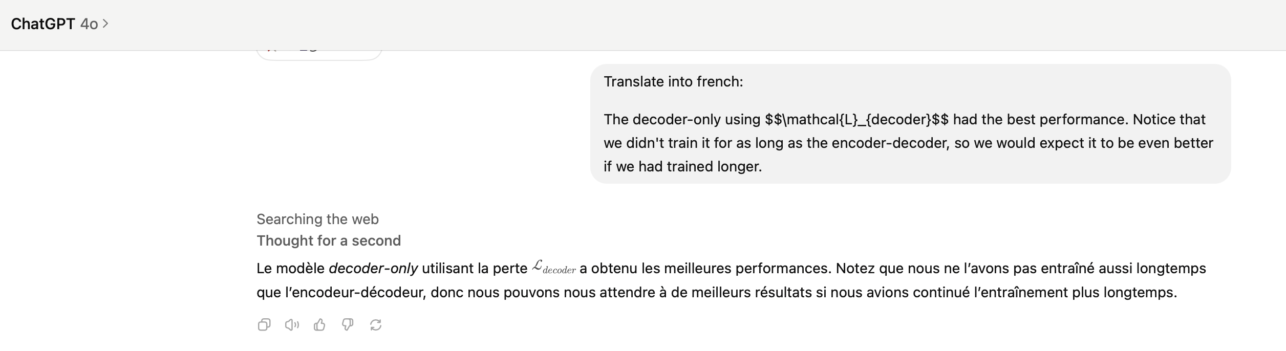
chatgpt translate — Figure 27: Example chatgpt translation

which when translated back to English via Google Translate yields:

The decoder-only model using the \mathcal{L}_{decoder} loss achieved the best performance. Note that we didn’t train it as long as the encoder-decoder, so we can expect better results if we had continued training for longer.

Attention weights

Finally, let’s look at some attention weights from the decoder-only model. The source text is given to the model as inference input, and the predicted tokens are iteratively added to the sequence. We collect the attention weights after completing the predicted sequence. Note that language tags <en> and <fr> are prepended to the english and French sequences respectively. Only showing weights > 0.1 to reduce the number of lines drawn.

We can see some interesting patterns. Here are ones that stand out as the most obvious.

Layer 1, head 2: Some tokens just pay attention to itself while others either pay attention to the same token output previously, e.g. “for” and “for” or the target token is aligned with the source token, e.g. “et” and “and”

Layer 5, head 5: Previous token attention

Layer 6, head 1: Tokens that go together are aligned, e.g. “si-mis-m” attend to “pes” or “tel” attend to “un” in “un tel” meaning “such”

Layer 9, head 3: Many tokens attend to <en> tag, which seems like a “default” or no-op that we’ve seen previously. This trend is repeated throughout many layers/heads, e.g., layer 18 head 5 attends to both <en> and <fr> respectively.

Overall, we see a mixture of the English sequence attending to its tokens, the French sequence attending to its tokens, and the French sequence attending to the English tokens. A significant number of layers/heads don’t contain useful signal and just attend to <en> and <fr>.

Conclusion

We’ve looked at the transformer architecture and how it differs from the RNN architecture that preceded it. The transformer has better performance on the translation task but beyond translation, is the SOTA model for multi-modal understanding and generation. It makes better use the hardware for parallelism and so is faster and more scalable than the RNN architecture. We also looked at how the original encoder-decoder transformer architecture compares to decoder-only LLM architecture and showed that the decoder-only model can achieve similar performance as the encoder-decoder on the original translation task as well. This shows that the original transformer could be formulated as a modern decoder-only transformer without loss in performance.

Excluding embedding layers ↩
The number of tokens processed is calculated as average tokens per iteration × number of iterations. ↩
Only including train time, not inference/validation ↩
FLOP calculation is $C=6ND$ per Kaplan et al. 2020 (see this blog post). ↩
WMT’14 test set BLEU ↩

The dominant sequence transduction models are based on complex recurrent or convolutional neural networks that include an encoder and a decoder. The best performing models also connect the encoder and decoder through an attention mechanism. We propose a new simple network architecture, the Transformer, based solely on attention mechanisms, dispensing with recurrence and convolutions entirely. Experiments on two machine translation tasks show these models to be superior in quality while being more parallelizable and requiring significantly less time to train. Our model achieves 28.4 BLEU on the WMT 2014 English-to-German translation task, improving over the existing best results, including ensembles, by over 2 BLEU. On the WMT 2014 English-to-French translation task, our model establishes a new single-model state-of-the-art BLEU score of 41.0 after training for 3.5 days on eight GPUs, a small fraction of the training costs of the best models from the literature.

Training Deep Neural Networks is complicated by the fact that the distribution of each layer’s inputs changes during training, as the parameters of the previous layers change. This slows down the training by requiring lower learning rates and careful parameter initialization, and makes it notoriously hard to train models with saturating nonlinearities. We refer to this phenomenon as internal covariate shift, and address the problem by normalizing layer inputs. Our method draws its strength from making normalization a part of the model architecture and performing the normalization for each training mini-batch. Batch Normalization allows us to use much higher learning rates and be less careful about initialization, and in some cases eliminates the need for Dropout. Applied to a state-of-the-art image classification model, Batch Normalization achieves the same accuracy with 14 times fewer training steps, and beats the original model by a significant margin. Using an ensemble of batch-normalized networks, we improve upon the best published result on ImageNet classification: reaching 4.82% top-5 test error, exceeding the accuracy of human raters.

Deeper neural networks are more difficult to train. We present a residual learning framework to ease the training of networks that are substantially deeper than those used previously. We explicitly reformulate the layers as learning residual functions with reference to the layer inputs, instead of learning unreferenced functions. We provide comprehensive empirical evidence showing that these residual networks are easier to optimize, and can gain accuracy from considerably increased depth. On the ImageNet dataset we evaluate residual nets with a depth of up to 152 layers - 8× deeper than VGG nets [40] but still having lower complexity. An ensemble of these residual nets achieves 3.57% error on the ImageNet test set. This result won the 1st place on the ILSVRC 2015 classification task. We also present analysis on CIFAR-10 with 100 and 1000 layers. The depth of representations is of central importance for many visual recognition tasks. Solely due to our extremely deep representations, we obtain a 28% relative improvement on the COCO object detection dataset. Deep residual nets are foundations of our submissions to ILSVRC & COCO 2015 competitions1, where we also won the 1st places on the tasks of ImageNet detection, ImageNet localization, COCO detection, and COCO segmentation.

References

- Attention is all you needIn Proceedings of the 31st International Conference on Neural Information Processing Systems, Long Beach, California, USA, Jun 2017
- Batch normalization: accelerating deep network training by reducing internal covariate shiftIn Proceedings of the 32nd International Conference on International Conference on Machine Learning - Volume 37, Lille, France, Jun 2015
- Layer NormalizationJun 2016
- Deep Residual Learning for Image RecognitionIn 2016 IEEE Conference on Computer Vision and Pattern Recognition (CVPR), Jun 2016
- On layer normalization in the transformer architectureIn Proceedings of the 37th International Conference on Machine Learning, Jun 2020
- What does Bert Look at? an analysis of Bert’s attentionJun 2019
- Scaling laws for neural language modelsJan 2020
- Bridging nonlinearities and stochastic regularizers with gaussian error linear unitsJun 2016
- Language models are good translatorsJun 2021
Enjoy Reading This Article?
Here are some more articles you might like to read next: